Introduction to Bayesian Analysis

library(tidyverse)
library(ggside)
library(hrbrthemes)
theme_set(theme_ipsum_rc())
set.seed(123)

ads_shown   = 100
conversion  = ads_shown * 0.13
n_samples   = 100e3

Frequentist Approach

# generate null distribution
n_converts <-
    rbinom(n = n_samples, size = ads_shown, prob = 0.10)

n_converts |> 
    data.frame() |> 
    ggplot(aes(x = n_converts)) +
    geom_histogram(col = "darkblue", fill = "lightblue", bins = 10) +
    geom_vline(xintercept = conversion, col = "red", lty = 4) +
    scale_y_comma() + 
    labs(x = "# Visitors", title = "Binom. Distribution")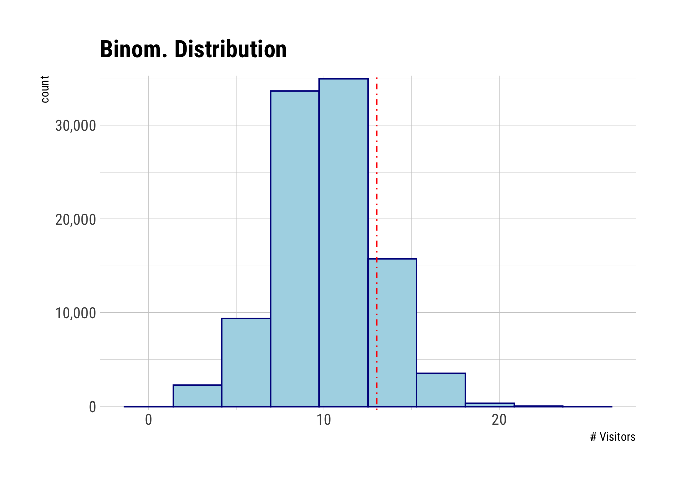

# calc prob
freq_prob <- sum(n_converts >= conversion) / length(n_converts)
freq_prob

## [1] 0.19748

# shortcut
1 - pbinom(conversion-1, size = ads_shown, prob = 0.10)

## [1] 0.1981789

Bayesian Approach

# given Bayesian way of doing, we expect a prior distribution
# assume expected CVR as a beta distribution

# params for beta distribution
ab = list(a = 11.3, b = 93.5)

prior_prop_clicks <- rbeta(n = n_samples, shape1 = ab$a, shape2 = ab$b)

prior_prop_clicks |>
    density() |>
    plot(
        type = "h",
        col  = "light blue",
        main = "Beta Distribution (Prior)"
    )

abline(v = 0.1, col = "red")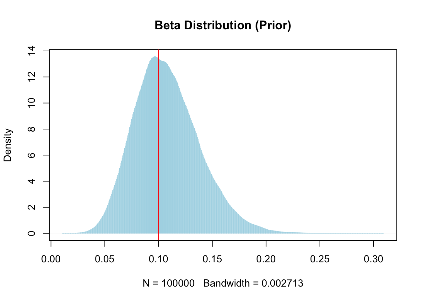

n_converts  <- rbinom(n = n_samples, size = ads_shown, prob = prior_prop_clicks)
prior       <- tibble(rate = prior_prop_clicks, visits = n_converts)

# visualize a joint probability distribution
prior |>
    ggplot(aes(visits, rate)) +
    geom_jitter(col = "lightblue", alpha = 0.05, width = 0.05) +
    geom_xsidehistogram(
        aes(y = stat(density)), 
        bins = 15, 
        col  = "darkblue",
        fill = "lightblue"
    ) +
    geom_ysidehistogram(
        aes(x = stat(density)), 
        bins = 15, 
        col  = "darkblue",
        fill = "lightblue"
    ) +
    labs(title = "Joint Distribution")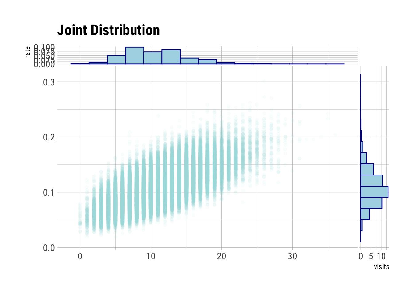

# calc prob
bayes_prob <- sum(n_converts >= conversion) / length(n_converts)
bayes_prob

## [1] 0.31883

prior |>
    filter(visits == conversion) |>
    ggplot(aes(rate)) +
    geom_histogram(aes(y = ..density..),
        col  = "white",
        fill = "lightblue",
        bins = 30
    ) +
    geom_density(col = "darkblue", size = 2) +
    coord_cartesian(xlim = c(0, .5)) +
    labs(title = "Posterior Distribution (New Prior)")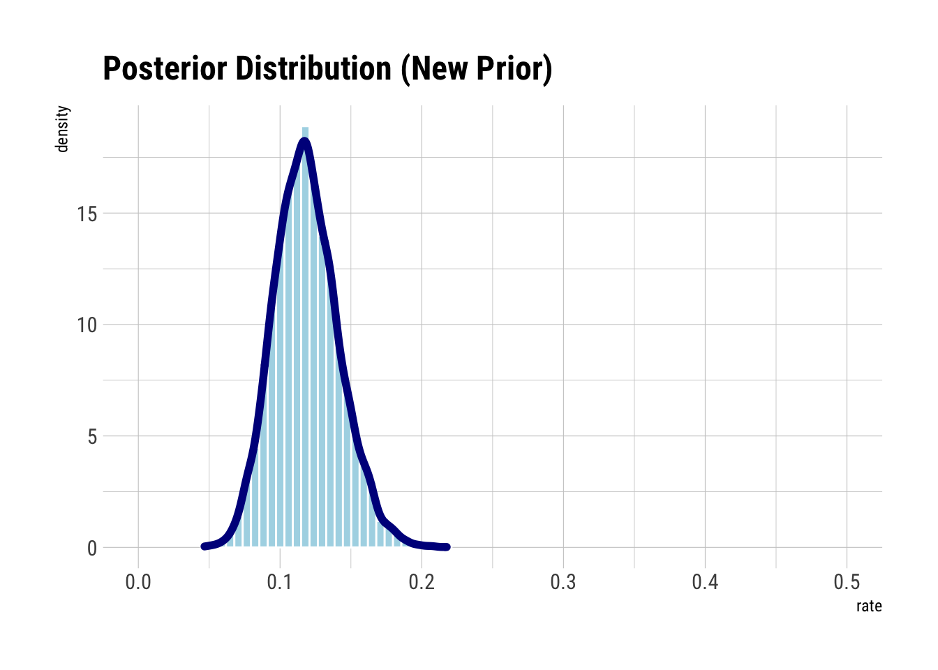

# posterior distribution can be used as a new prior 
posterior <- prior |> filter(visits == conversion) |> pull(rate)
mean(posterior)

## [1] 0.1186554

Given its prior, Bayesian > Frequentist.

# to compare
list(
    frequentist = freq_prob,
    bayesian    = bayes_prob
)

## $frequentist
## [1] 0.19748
## 
## $bayesian
## [1] 0.31883

Decision Analysis

Compare cost-benefit to SEM getting 7/80. Assume SEM’s average conversion is 8% with sigma 1%. Cost for ads is $500, cost for SEM is $400.

sem_impressions = 80
sem_converts    = 7

# assume prior
sem_prior_prob <- rnorm(n = n_samples, mean = 0.08, sd = 0.01)

sem_prior_prob |> 
    density() |> 
    plot(
        type = "h",
        col  = "orange",
        main = "Normal Distribution (Prior)"
    )

abline(v = 0.08, col = "red")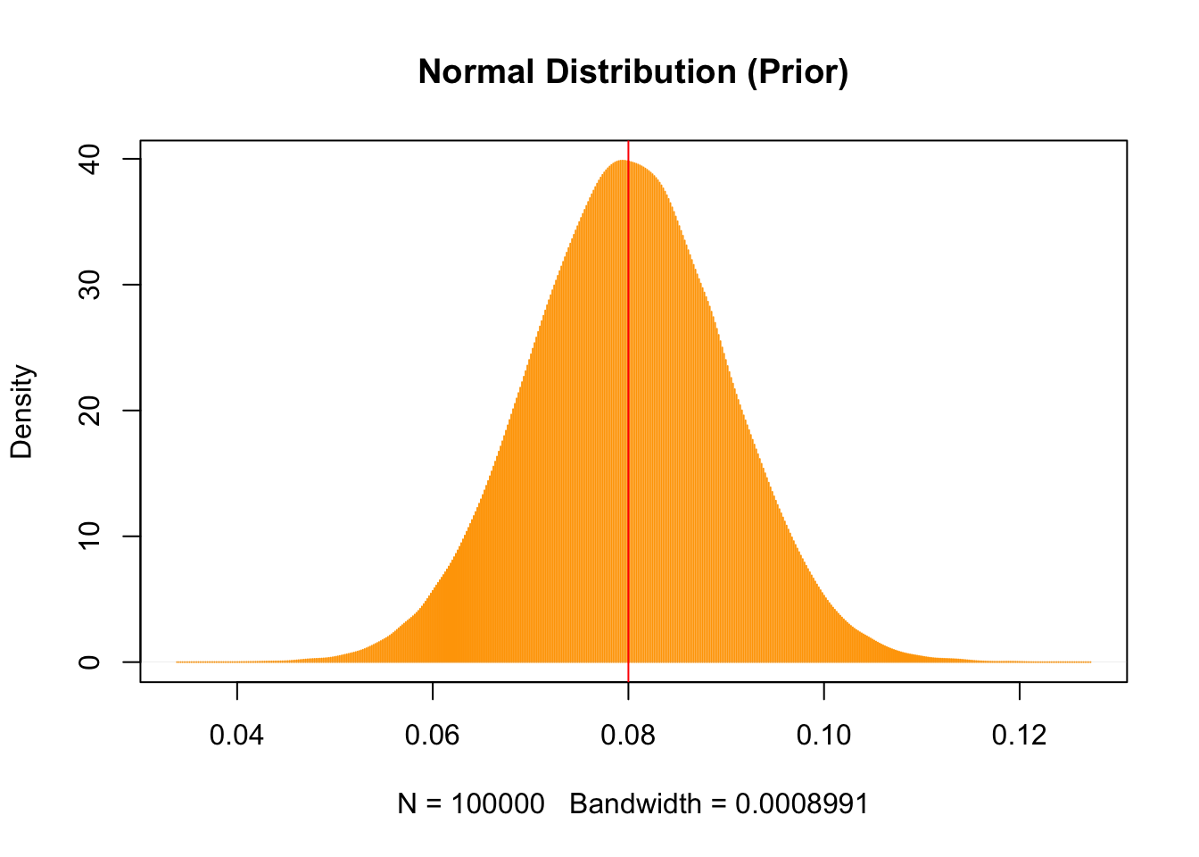

sem_prior <- rbinom(n = n_samples, size = sem_impressions, prob = sem_prior_prob)
sem_prior <- tibble(rate = sem_prior_prob, convert = sem_prior)

sem_prior |>
    filter(convert == sem_converts) |>
    ggplot(aes(rate)) +
    geom_histogram(aes(y = ..density..),
        col   = "white",
        fill  = "orange",
        bins  = 30,
        alpha = 0.3
    ) +
    geom_density(col = "darkorange", size = 2) +
    coord_cartesian(xlim = c(0, .5)) +
    labs(title = "Posterior for SEM")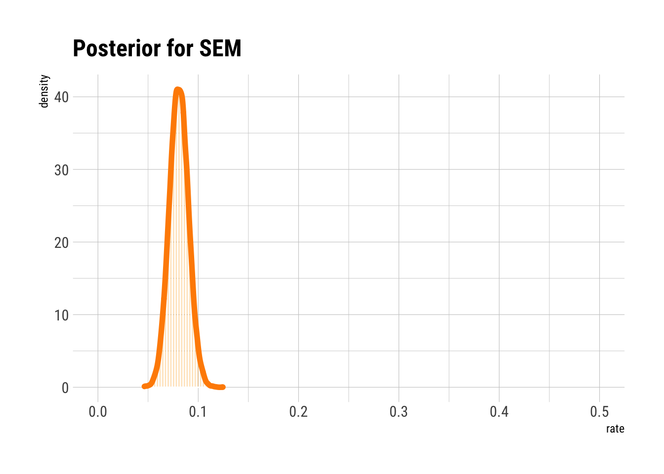

sem_posterior <- 
    sem_prior |> 
    filter(convert == sem_converts) |> 
    pull(rate)
mean(sem_posterior)

## [1] 0.08076218

df <- tibble(
    ad_converts  = rbinom(n = n_samples, size = ads_shown, prob = posterior),
    sem_converts = rbinom(n = n_samples, size = sem_impressions, prob = sem_posterior),
    ad_cost      = ad_converts  * 500,
    sem_cost     = sem_converts * 400,
    cost_diff    = ad_cost - sem_cost
)

df |> 
    ggplot(aes(cost_diff)) + 
    geom_histogram(bins = 30, fill = "cyan", col = "black", alpha = 0.3) +
    geom_vline(xintercept = 0, lty = 4, col = "red") +
    scale_x_continuous(labels = scales::dollar) +
    scale_y_comma() + 
    labs(x = "Cost Diff. (Ads - SEM)", title = "Compare Ads to SEM")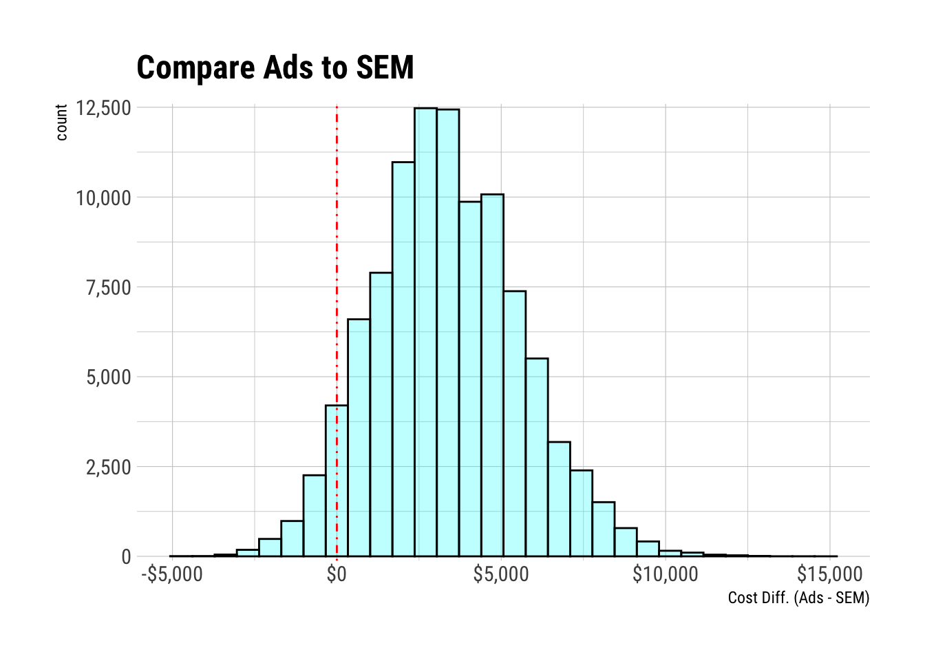

# prob of ads is better
df |> summarise(prob = sum(cost_diff < 0) / n())

## # A tibble: 1 × 1
##     prob
##    <dbl>
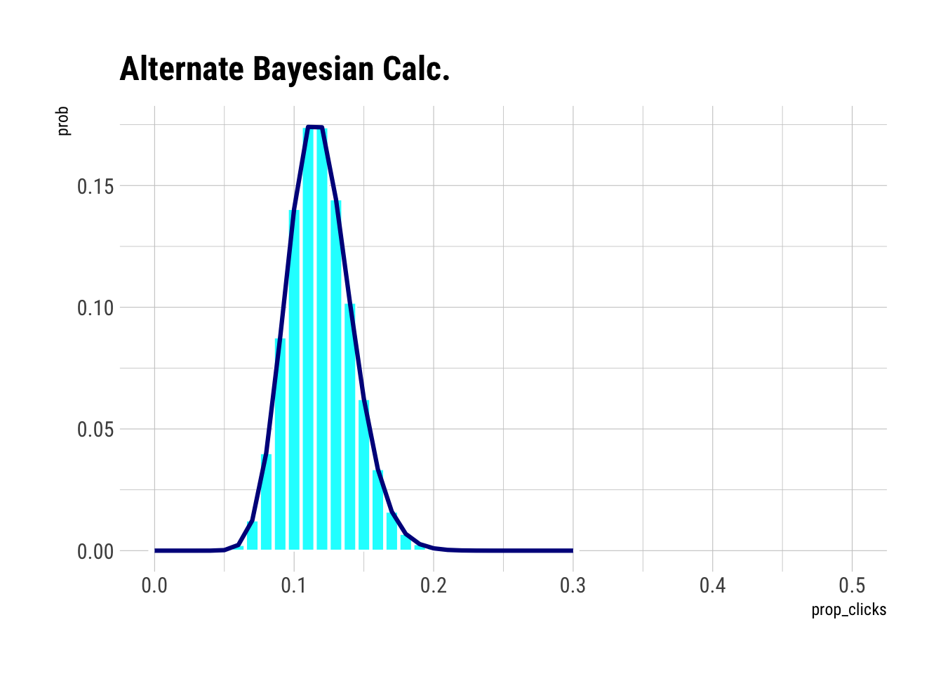
## 1 0.0551

Shortcut to Bayesian Calculation

Use density d instead of drawing samples r.

calc <- tibble(
    prop_clicks  = seq(0, .3, by = 0.01),
    prior        = dbeta(prop_clicks, shape1 = ab$a, shape2 = ab$b),
    likelihood   = dbinom(conversion, size = ads_shown, prob = prop_clicks),
    prob         = prior * likelihood
) |>
    mutate(prob = prob / sum(prob))

calc |> 
    ggplot(aes(prop_clicks, prob)) + 
    geom_col(col = "white", fill = "cyan") + 
    geom_line(col = "dark blue", size = 1.1) + 
    coord_cartesian(xlim = c(0, .5)) +
    labs(title = "Alternate Bayesian Calc.")