Spam Attack: A Yule Process Simulation

May 6, 2020 #stochastic

From 538’s The Riddler,

Over the course of three days, suppose the probability of any spammer making a new comment on this week’s Riddler column over a very short time interval is proportional to the length of that time interval. (For those in the know, I’m saying that spammers follow a Poisson process.)
On average, the column gets one brand-new comment of spam per day that is not a reply to any previous comments. Each spam comment or reply also gets its own spam reply at an average rate of one per day. For example, after three days, I might have four comments that were not replies to any previous comments, and each of them might have a few replies (and their replies might have replies, which might have further replies, etc.).
After the three days are up, how many total spam posts (comments plus replies) can I expect to have?

library(tidyverse)
library(furrr)
library(ggforce)
set.seed(1234)
future::plan(strategy = "multiprocess")

N = 300
trials = 1e5

# this is our answer to question above
x = replicate(trials, sum(cumsum(rexp(n = N, rate = 1:N)) < 3))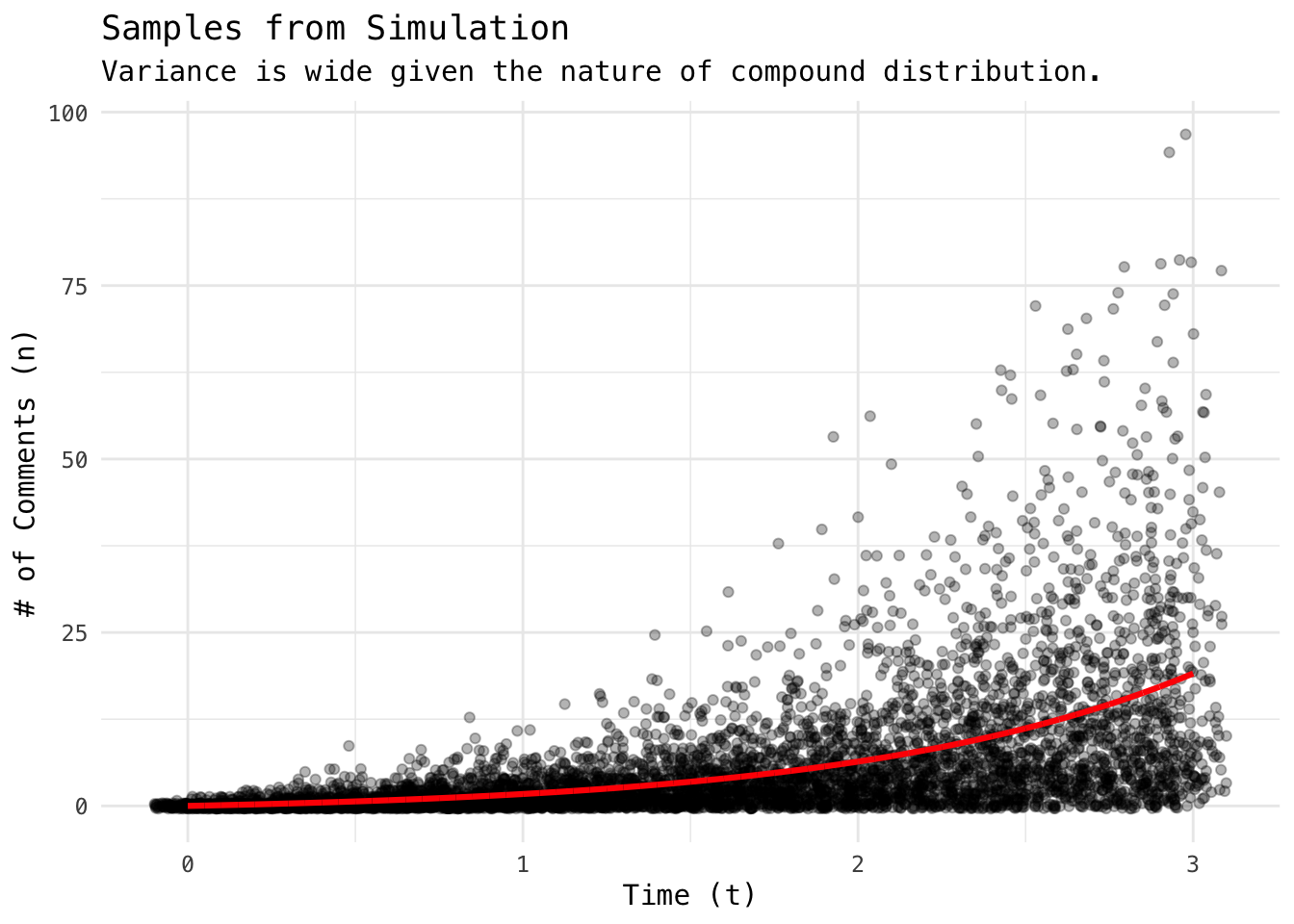
mean(x, na.rm = TRUE)

## [1] 19.08135

We can further investigate the growth of spam comments to highlight the fact that using average (as expected value) in a compound distribution is usually not a good idea. The spread (variance) can be extremely large.

# further simulate possible 'growth' by every 3-minutes
seqs = seq(0, 3, 0.05)
res  = furrr::future_map_dbl(rep(seqs, trials), ~ sum(cumsum(rexp(n = N, rate = 1:N)) < .x))

res_df <- tibble(
    trial    = rep(1:trials, each = length(seqs)),
    t        = rep(seqs, trials),
    comments = res
)

# compute mean of trials
res_df %>% 
    group_by(t) %>% 
    summarise(mu = mean(comments)) %>% 
    ggplot(aes(t, mu)) + 
    geom_line(size = 1.2) + 
    geom_mark_circle(aes(label = mu, filter = t == 3), 
                     col = "red", expand = unit(10, "mm")) +
    theme_minimal(base_family = "Menlo") +
    labs(x        = "Time (t)", 
         y        = "Expected # of Comments (n)",
         title    = "A Stochastic Simulation to Spam Comments",
         subtitle = "Result shows a function of exp(t) - 1.")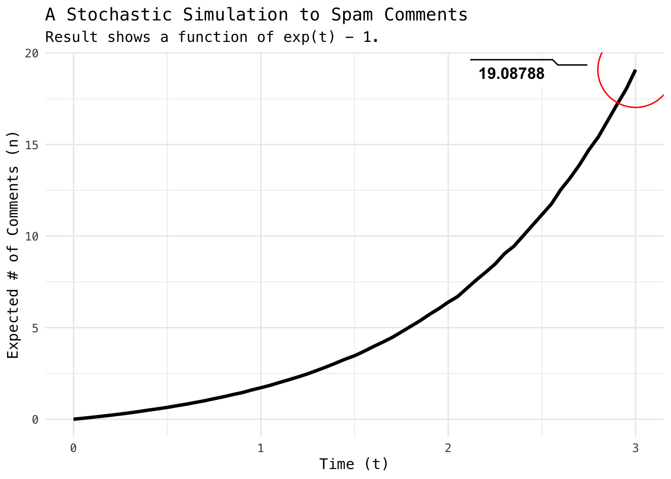

# sample some data to display variance
res_df %>% 
    filter(trial %in% sample(trials, 100)) %>% 
    ggplot(aes(t, comments)) + 
    geom_point(position = position_jitter(0.1), alpha = 0.3) + 
    geom_line(aes(y = exp(t) - 1), col = "red", size = 1.1) +
    theme_minimal(base_family = "Menlo") + 
    labs(x        = "Time (t)", 
         y        = "# of Comments (n)",
         title    = "Samples from Simulation",
         subtitle = "Variance is wide given the nature of compound distribution.")