STM Package Walkthrough Part Two
Apr 5, 2020 #topic-model #stm
This is our working data.
library(stm)## stm v1.3.5 successfully loaded. See ?stm for help.
## Papers, resources, and other materials at structuraltopicmodel.comdplyr::glimpse(dat)## Observations: 13,246
## Variables: 5
## $ documents <chr> "After a week of false statements, lies, and dismissiv…
## $ docname <chr> "at0800300_1.text", "at0800300_2.text", "at0800300_3.t…
## $ rating <chr> "Conservative", "Conservative", "Conservative", "Conse…
## $ day <int> 3, 3, 3, 3, 3, 3, 4, 4, 4, 4, 4, 4, 4, 4, 4, 5, 5, 5, …
## $ blog <chr> "at", "at", "at", "at", "at", "at", "at", "at", "at", …First ingest and prepare documents.
processed <- textProcessor(dat$documents, metadata = dat)## Building corpus...
## Converting to Lower Case...
## Removing punctuation...
## Removing stopwords...
## Removing numbers...
## Stemming...
## Creating Output...out <-
prepDocuments(processed$documents,
processed$vocab,
processed$meta,
lower.thresh = 10)## Removing 111851 of 123990 terms (189793 of 2298953 tokens) due to frequency
## Your corpus now has 13246 documents, 12139 terms and 2109160 tokens.stm package has a built-in function searchK to assist in selecting the best K parameter for topic modeling.
storage <- searchK(
    documents  = out$documents,
    vocab      = out$vocab,
    K          = c(15:25),
    cores      = 8, ## parallel computing
    prevalence =  ~ rating + s(day),
    data       = out$meta
)
Measures:
Semantic Coherence - related to pointwise mutual information (Mimno et al 2011). In models that are semantically coherent, words which are most probable under a topic should co-occur within the same document.
Exclusivity - based on FREX, weighted harmonic mean of the word’s rank in terms of exclusivity and frequency.
Heldout Likelihood - hold out some fraction of the words in training and use the document-level latent variables to evaluate the probability of the heldout portion.
Bound - The change in the approximate variational lower bound to convergence.
Residuals - multinomial dispersion of the STM residuals σ2=1. If we calculate the sample dispersion and the value is greater than one, this implies that K is set too low.
storage$results## K exclus semcoh heldout residual bound lbound em.its
## 1 15 9.533329 -66.29118 -7.534990 4.197934 -21753405 -21753377 49
## 2 16 9.533826 -67.45197 -7.521909 4.127972 -21720675 -21720644 58
## 3 17 9.598133 -68.89567 -7.518219 4.071788 -21704477 -21704443 51
## 4 18 9.578377 -68.37388 -7.511707 4.035990 -21690165 -21690129 33
## 5 19 9.594316 -69.40491 -7.505795 3.989638 -21671165 -21671126 44
## 6 20 9.573621 -71.09860 -7.501179 3.941228 -21651145 -21651103 31
## 7 21 9.585543 -71.78739 -7.495623 3.891438 -21627507 -21627462 27
## 8 22 9.602845 -71.27387 -7.487177 3.875203 -21609256 -21609207 42
## 9 23 9.613775 -75.72488 -7.478085 3.853901 -21582873 -21582822 49
## 10 24 9.626096 -74.62884 -7.475701 3.818413 -21569228 -21569173 46
## 11 25 9.671310 -74.40441 -7.467765 3.815041 -21545405 -21545347 71library(dplyr)
library(ggplot2)
library(ggforce)
old <-
theme_set(theme_minimal(base_family = "Menlo") +
theme(axis.text.x = element_text(angle = 90)))
df <- storage$results %>% mutate(K = as.factor(K))
df %>%
ggplot(aes(K, semcoh, group = 1)) +
geom_line() +
labs(x = "", y = "", title = "Semantic Coherence")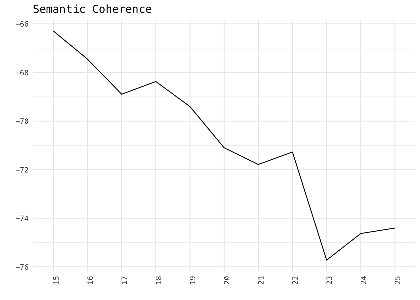
df %>%
    ggplot(aes(K, heldout, group = 1)) +
    geom_line() +
    labs(x = "", y = "", title = "Heldout Prob.")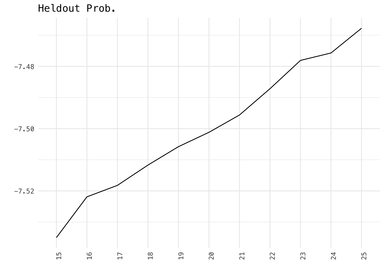
df %>%
    ggplot(aes(K, residual, group = 1)) +
    geom_line() +
    labs(x = "", y = "", title = "Residuals")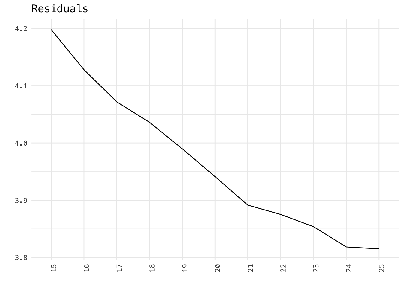
df %>%
    ggplot(aes(semcoh, exclus, col = K)) +
    geom_point(size = 3) +
    geom_mark_circle(aes(filter = K %in% c(17, 19, 22)),
                     col = "red", description = "Potentials best candidates for K") +
    labs(x = "Semantic Coherence", y = "Exclusivity") +
    theme(legend.position = "bottom")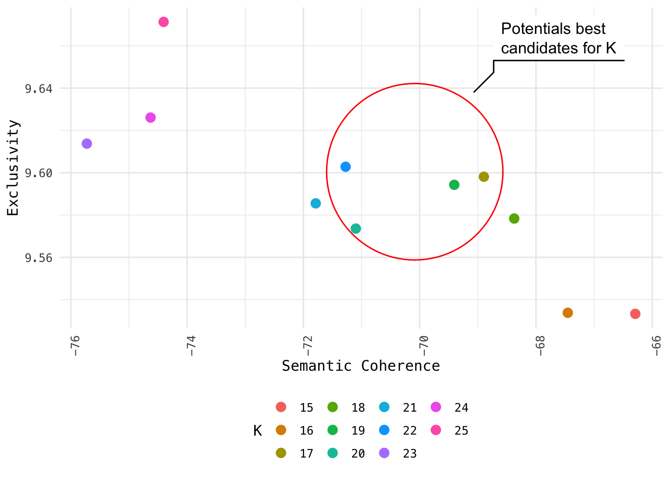
We have narrowed the range of K and may proceed to do further inspection via other techniques.