STM Package Walkthrough Part One

library(stm)
library(stmCorrViz)

## Observations: 13,246
## Variables: 5
## $ documents <chr> "After a week of false statements, lies, and dismissiv…
## $ docname   <chr> "at0800300_1.text", "at0800300_2.text", "at0800300_3.t…
## $ rating    <chr> "Conservative", "Conservative", "Conservative", "Conse…
## $ day       <int> 3, 3, 3, 3, 3, 3, 4, 4, 4, 4, 4, 4, 4, 4, 4, 5, 5, 5, …
## $ blog      <chr> "at", "at", "at", "at", "at", "at", "at", "at", "at", …

3.1. Ingest: Reading and processing text data

# produce word indices and their associated counts
processed <- textProcessor(dat$documents, metadata = dat)

## Building corpus... 
## Converting to Lower Case... 
## Removing punctuation... 
## Removing stopwords... 
## Removing numbers... 
## Stemming... 
## Creating Output...

length(processed$documents) == nrow(dat)

## [1] TRUE

# plot documents, words and tokens removed at various word thresholds
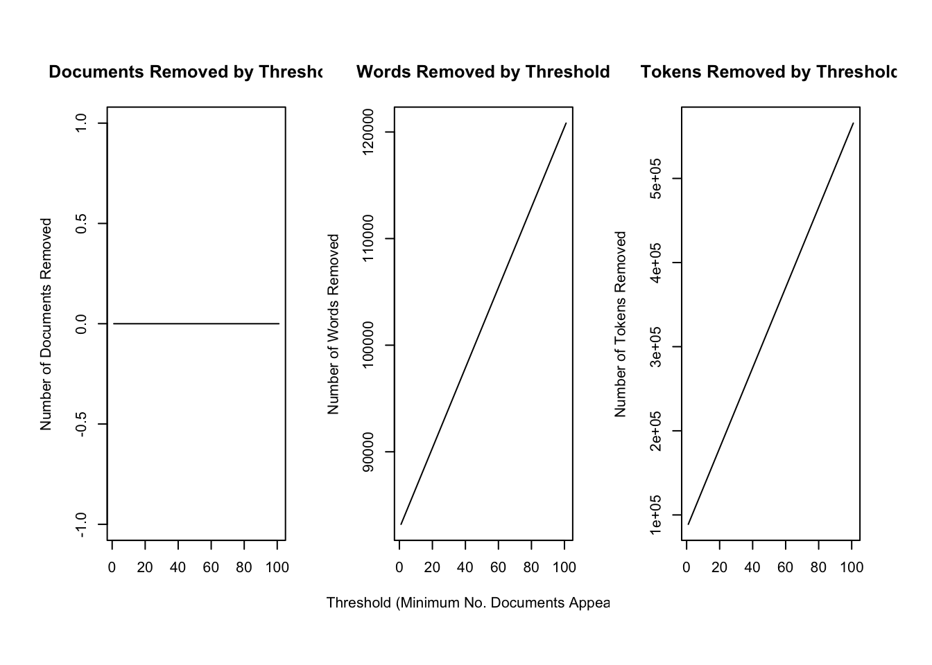
plotRemoved(processed$documents, lower.thresh = seq(1, 200, by = 100))

3.2 Prepare: Associate text with metadata

out   <- prepDocuments(processed$documents, processed$vocab, processed$meta, lower.thresh = 10)

## Removing 111851 of 123990 terms (189793 of 2298953 tokens) due to frequency 
## Your corpus now has 13246 documents, 12139 terms and 2109160 tokens.

3.3 Estimate: Estimating the structural topic model

poliblogPrevFit <-
    stm(
        documents = out$documents,
        vocab = out$vocab,
        K = 20,
        prevalence =  ~ rating + s(day),
        max.em.its = 75,
        data = out$meta,
        init.type = "Spectral",
        seed = 8458159
    )

3.4 Evaluate: Model selection and search

not included here (see part 2)

3.6. Visualize: Presenting STM results

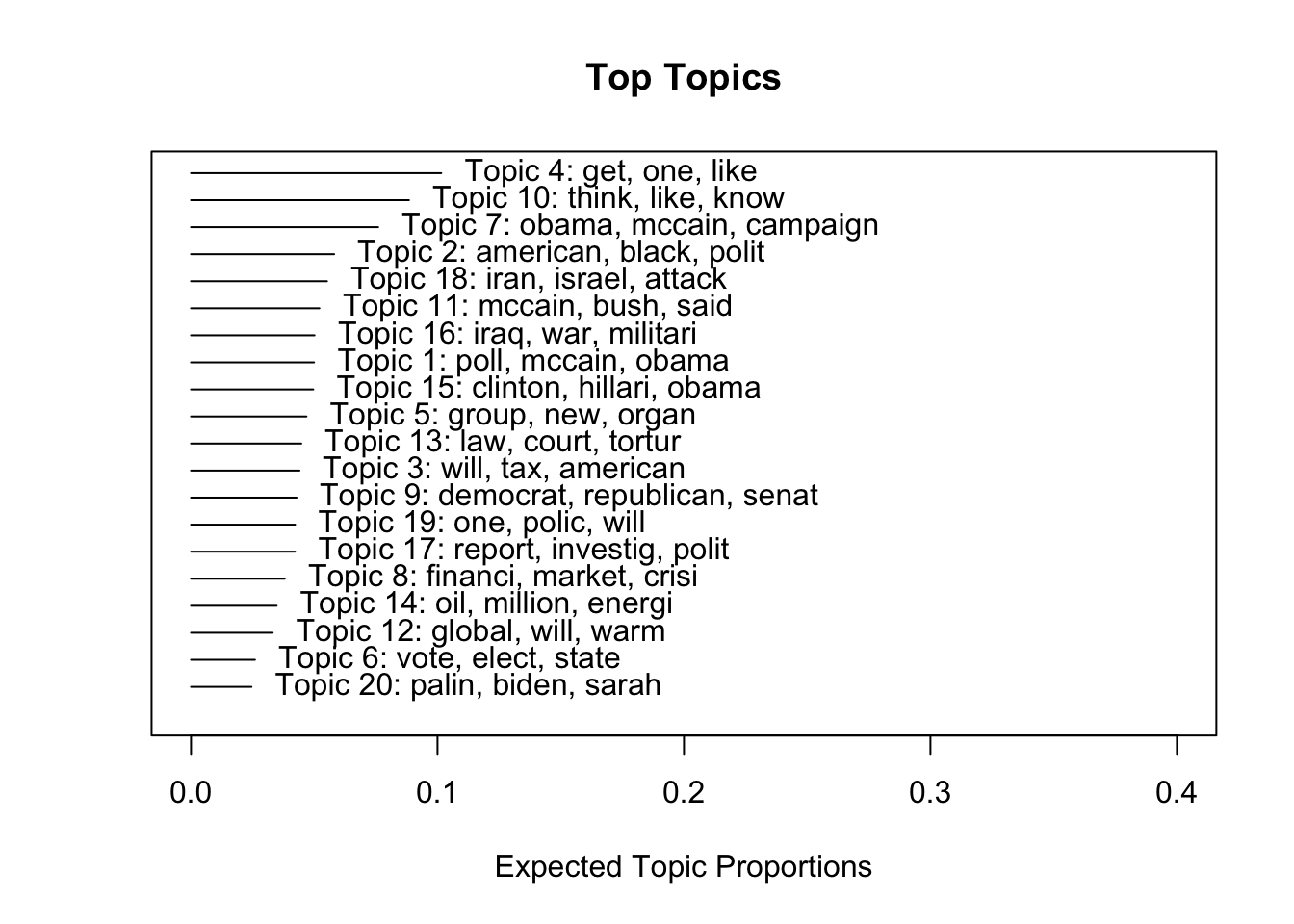
plot(poliblogPrevFit, type = "summary", xlim = c(0, .4))

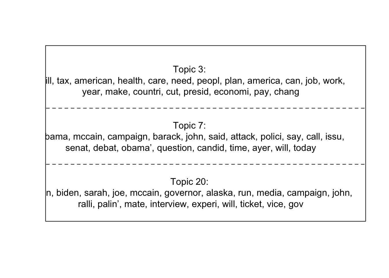
plot(poliblogPrevFit, type = "labels", topics = c(3, 7, 20))

Interactive visual via stmCorrViz package.

# NOT RUN 
stmCorrViz(
    mod = poliblogPrevFit,
    file_out = "stm-interactive-correlation.html",
    documents_raw = dat$documents,
    documents_matrix = out$documents
)