Puzzle: The Riddler Feb 21 - Coin Flipping Madness

Mar 13, 2020 #monte-carlo #dynamic

You have two fair coins, labeled A and B. When you flip coin A, you get 1 point if it comes up heads, but you lose 1 point if it comes up tails. Coin B is worth twice as much — when you flip coin B, you get 2 points if it comes up heads, but you lose 2 points if it comes up tails.

To play the game, you make a total of 100 flips. For each flip, you can choose either coin, and you know the outcomes of all the previous flips. In order to win, you must finish with a positive total score. In your eyes, finishing with 2 points is just as good as finishing with 200 points — any positive score is a win. (By the same token, finishing with 0 or −2 points is just as bad as finishing with −200 points.)

If you optimize your strategy, what percentage of games will you win? (Remember, one game consists of 100 coin flips.)

library(purrr)
library(furrr)

# flipping coin A or B with respective points
flip_coin <- function(coin) {
    x = ifelse(rbinom(1, 1, 0.5), 1, -1)
    ifelse(coin == "A", x * 1, x * 2)
}

# acc = accumulative score; i = remaining flip;
run_game <- function(acc, i, threshold = 0) {
    
    # terminal condition
    if (i == 0) return(acc);
    
    ## this is our strategy: 
    ## only when we're behind taking risk makes a difference
    x = ifelse(acc < threshold, flip_coin("B"), flip_coin("A"))
    
    run_game(acc + x, i - 1, threshold)
}

set.seed(1111)
trials = 3000
res = replicate(trials, run_game(0, 100))
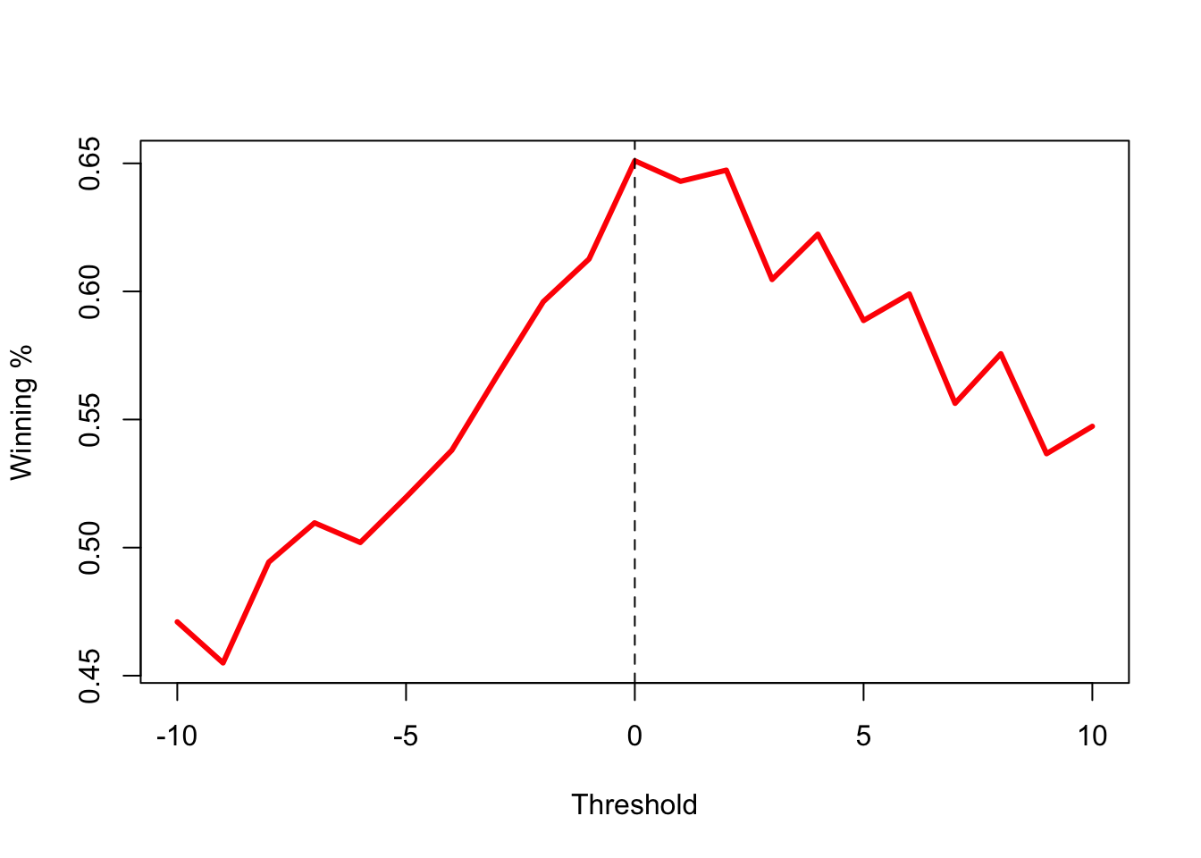
sum(res > 0) / trials # win game if positive

## [1] 0.6366667

The answer is 64%. If you play the game the optimal way, you are able to win ~64% of the time. Here, we vary the threshold to adjust the strategy from conservative (-10) to aggresive mode (10). Also note that, if you choose your strategy to only play either coin A or coin B, your winning probability is only 46% instead of 50% (because zero is considered a loss).

# prepare for parellel computation
future::plan(multiprocess)

thres <- -10:10
res <- furrr::future_map_dbl(thres, ~ {
  mean(replicate(trials, run_game(0, 100, threshold = .x)) > 0)
})

plot(thres, res, type = "l", lwd = 3, col = "red",
     xlab = "Threshold", ylab = "Winning %")
abline(v = 0, lty = 2)

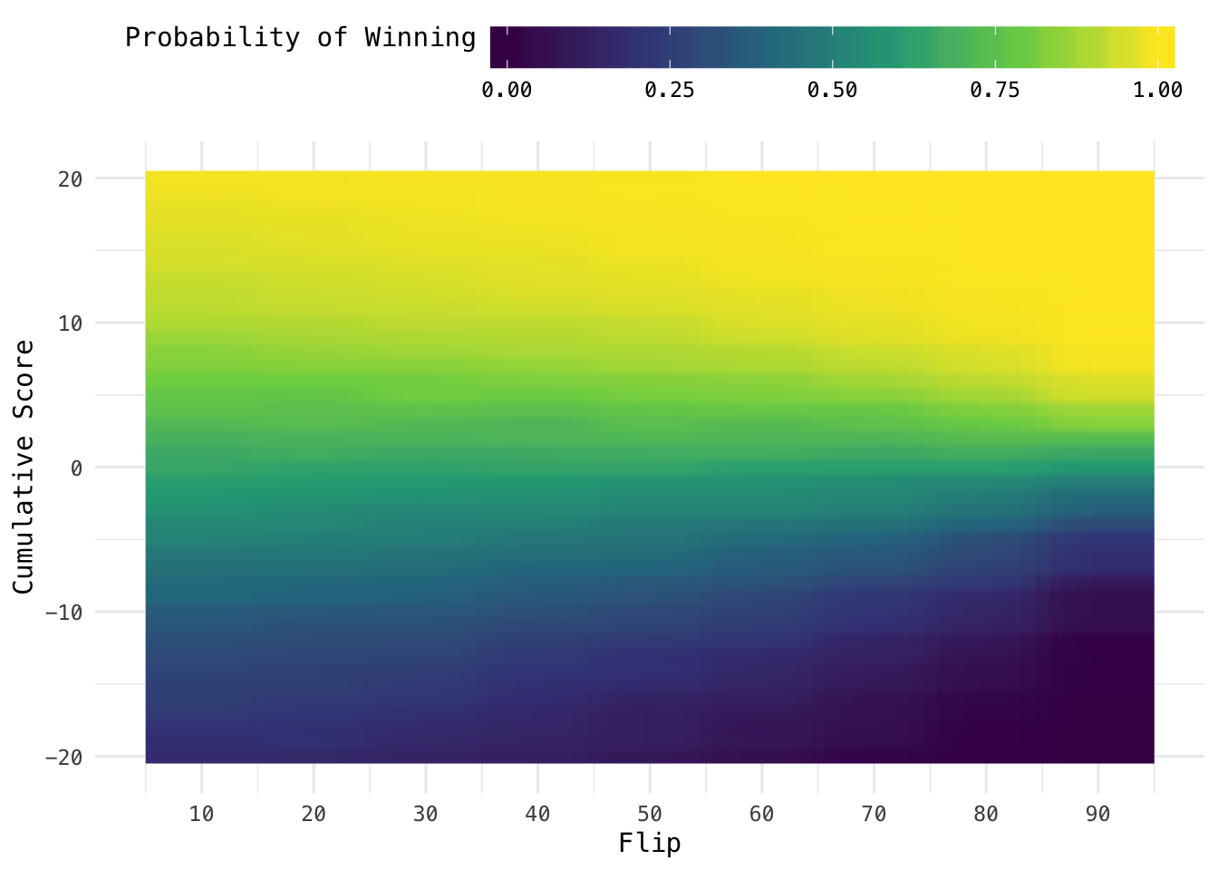
For further analysis, we can explore the winning chances at any point of in the game. For an instance, if you are left with 10 flips and are 5 points behind, what are the odds of you winning the game at the end?

# create a data frame as grid for simulation
df <- expand.grid(remaining = seq(10, 90, 10), acc = seq(-20, 20, 1))

# a point on grid represents a single possibility
# loop thru our grid to calc expected chances
res <- future_map2_dbl(df$acc, df$remaining, ~ {
    sum(replicate(trials, run_game(.x, .y)) > 0) / trials
})

We use a heat map to illustrate this.

library(ggplot2)

df %>%
  # attach winning chances
  cbind(prob = res) %>%
  ggplot(aes(100 - remaining, acc)) +
  # take note of interpolation here
  geom_raster(aes(fill = prob), interpolate = TRUE) +
  scale_x_continuous(breaks = seq(0, 100, 10)) +
  scale_fill_viridis_c() +
  theme_minimal(base_family = "Menlo") +
  theme(
    legend.position  = "top",
    legend.key.width = unit(2, "cm"),
    legend.title     = element_text(vjust = 1.0)
  ) +
  labs(x = "Flip", y = "Cumulative Score",
       fill = "Probability of Winning")