Puzzle: Blackjack Simulation

Feb 19, 2020 #monte-carlo

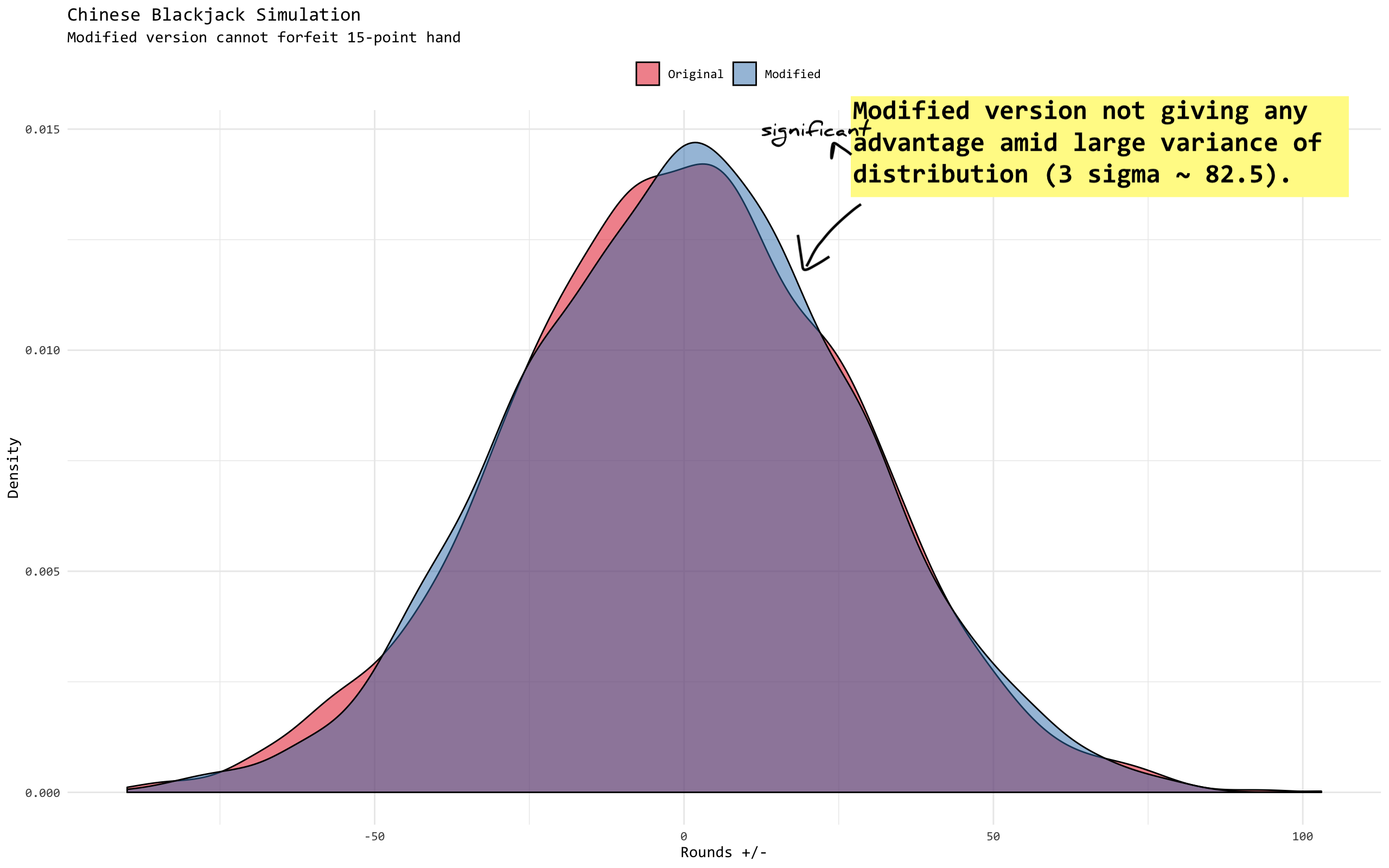
A game of Chinese BlackJack is played by N players where one of them being the dealer. Normally, any player except the dealer can choose to forfeit the round if they get 15-point (free-hand) dealt. However, in this occasion everyone agrees that 15-point is not allowed to forfeit and must continue to draw. Common sense tells us that the probability of picking a card more than 6 (go bust for player) is \(\frac{52-24-1}{52-2}\) or 54% thus giving a dealer an upper edge. The question here, is the upper edge significant enough?

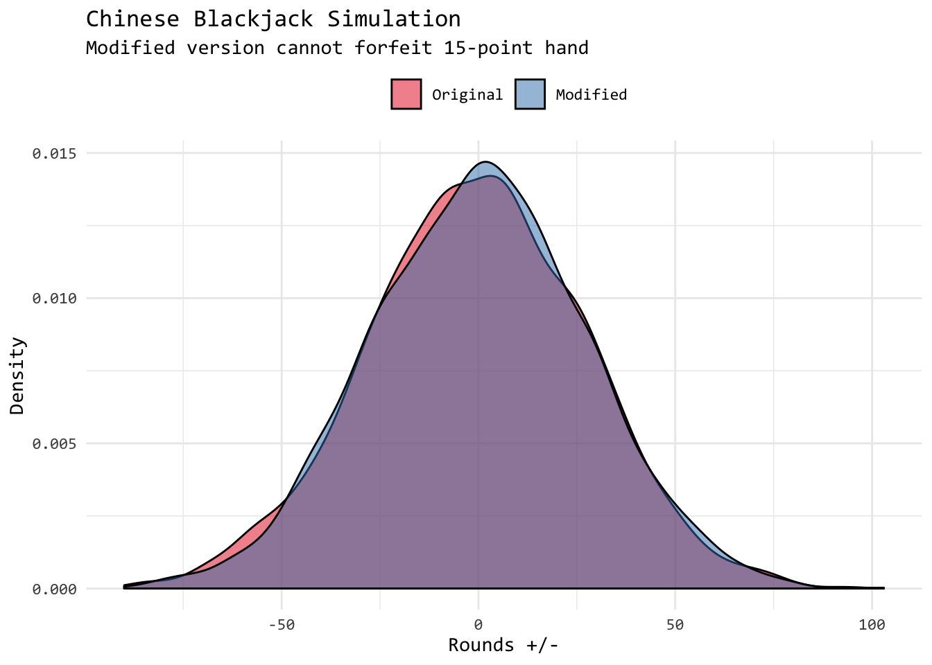
Well, not really. The fact that the game itself inherits large uncertainty, adding that probabilistic advantage won’t make a difference. Note, the x-axis here is win or lose game round, not equity (cash value).

Perhaps this serves as another reminder. In this complex world, relative advantage is not the same as absolute advantage. Very often, chaos and randomness dominate more than anything else. It is like there are so many finance and economics PhDs out there trying to beat the market. It is not entirely impossible, but literally only a handful of people manage to accomplish that. And they don’t go by the book.

Code used for simulation written in R.

library(tidyverse)

# make a deck and shuffle
shuffle_deck <- function() {
    # ace(1) to nine + 10-point card (10, J, Q, K) 
    # suite is irrelevant
    c(rep(1:9, 4), rep(10, 4 * 4)) %>% sample(52) %>% as.integer()
}
dd <- shuffle_deck()

is_blackjack <- function(hh) {
    if (length(hh) != 2L) {
        stop("Length of hand does not make sense")
    }
    case_when(
        hh[1] == 1L  && hh[2] == 1L  ~ TRUE,
        hh[1] == 1L  && hh[2] == 10L ~ TRUE,
        hh[1] == 10L && hh[2] == 1L  ~ TRUE,
        TRUE ~ FALSE
    )
}

count_point  <- function(...) {
    if (any(... == 1L)) {
        addsome <- case_when(
            length(...) == 2L ~ 10,
            length(...) == 3L && sum(...) < 13 ~ 9,
            TRUE ~ 0
        )
        sum(...) + addsome
    } else {
        sum(...)
    }
}

check_hand   <- function(hand) {
    # browser()
  
    # check for blackjack first
    if (is_blackjack(hand[1:2])) {
      return(99L)
    }
    pos <- map_dbl(2:5, ~ count_point(hand[1:.x]))
    
    # check for 5-card charlie
    if (pos[4] <= 21) {
      return(99L)
    }
    
    # this is 5-card and bust
    if (pos[3] < 15 & pos[4] > 21) {
      return(0L)
    }
    
    # opt for risk-averse play 
    fin <- which(pos > 15 & pos <= 21)
    
    if (length(fin) > 1L) {
      pos[fin[1]]
    } else if (length(fin) == 1L) {
      pos[fin]
    } else {
      0L # bust
    }
}

run_game <- function(f, N = 5) {
  
  players = rep(1:N, N)
  
  dck <- shuffle_deck()
  
  hnd <- c(1:N) %>% map_dbl( ~ check_hand(dck[which(players == .x)]))
  
  f(hnd[1], hnd[-1])
  
}

calc_winloss_orig <- function(dealer, therest) {
  
  # compare players' card to dealer's
  wl <- map_dbl(therest,
                # original version player can forfeit 15
                ~ case_when(.x == 15 ~ 0,
                            dealer >  .x ~ 1,
                            dealer == .x ~ 0,
                            dealer <  .x ~ -1))
  
  # return dealer's win-loss
  sum(wl)
  
}

calc_winloss_new <- function(dealer, therest) {
  wl <- map_dbl(therest,
                ~ case_when(dealer >  .x ~ 1,
                            dealer == .x ~ 0,
                            dealer <  .x ~ -1))
  sum(wl)
}

# take nn games as one session
simulate_orig <- function(nn = 100) {
  sum(replicate(nn, run_game(calc_winloss_orig)))
}
simulate_new <- function(nn = 100) {
  sum(replicate(nn, run_game(calc_winloss_new)))
}

library(progress)

trials   = 3000
set_new  = numeric(trials)
set_orig = numeric(trials)
pb       = progress_bar$new(total = trials)

# this is going to take quite some time
for (i in 1:trials) {
  pb$tick()
  set_new[i]  <- simulate_new()
  set_orig[i] <- simulate_orig()
}

df <- tibble(orig = set_orig, new = set_new) %>% gather(set, val)

df %>%
  mutate(set = factor(set, levels = c("orig", "new"))) %>% 
  ggplot(aes(val, fill = set)) +
  geom_density(alpha = .5) +
  scale_fill_brewer(palette = "Set1", 
                    labels = c(orig = "Original",
                               new  = "Modified")) +
  theme_minimal(base_family = "Consolas") +
  theme(legend.position = "top") +
  labs(x     = "Rounds +/-", 
       y     = "Density",
       fill  = "",
       subtitle = "Modified version cannot forfeit 15-point hand",
       title = "Chinese Blackjack Simulation")

library(infer)

df %>% 
  group_by(set) %>% 
  summarise(mean = mean(val))

## # A tibble: 2 x 2
##   set     mean
##   <chr>  <dbl>
## 1 new    0.142
## 2 orig  -0.494

# use bootstrap inference to determine confidence interval
df %>% 
  specify(val ~ set) %>% 
  generate(reps = 3000, type = "bootstrap") %>% 
  calculate(stat = "diff in means", order = c("orig", "new")) %>% 
  summarise(l = quantile(stat, 0.025),
            m = median(stat),
            h = quantile(stat, 0.975))

## # A tibble: 1 x 3
##       l      m     h
##   <dbl>  <dbl> <dbl>
## 1 -2.00 -0.654 0.708