Simulate Customer Retention

Feb 28, 2019 #survival

The code below simulate a scenario where nc customers onboard during a ts timespan. However, none of them managed to retain for more than sp periods. The objective is to compare various customer retention analysis especially periodic and retrospective analysis techniques.

library(tidyverse)
library(charlatan)

# Generate Some Samples  ----------------------------------------------

# seeding
set.seed(123)

# number of customers
nc = 500
# timespan (entire periods)
ts = 1:12
# survival periods
sp = 3

# generate some customers data
cust_info <- data_frame(
  id = paste0("KB", ch_integer(n = nc, min = 100)),
  jobs = sample(ch_job(n = 4, locale = "zh_TW"), 
                size = length(id), replace = TRUE)
)

# generate a sequence of vector with length n 
make_seq <- function(n, x) {
  
  # initiate an empty vector
  vec = rep(0, n)
  
  # generate index with range no more than x
  ind = 1 : (2 + x)
  while(diff(range(ind)) > x) {
    ind = runif(x, 1, n + 1)
  }
  
  # fill vector with 1s 
  vec[ind] <- 1
  
  return(vec)
}
  
# repeats ts times
surv_times <- nc %>% 
  replicate(make_seq(max(ts), sp)) %>% 
  t() %>% as_data_frame()
names(surv_times) <- paste0("M", ts)

# calc initial register period
join <- apply(surv_times, 1, function(x) min(which(x == 1)))

# samples 
dat <- bind_cols(cust_info, join = join, surv_times)
head(dat)  

## # A tibble: 6 x 15
##   id    jobs    join    M1    M2    M3    M4    M5    M6    M7    M8    M9   M10
##   <chr> <chr>  <int> <dbl> <dbl> <dbl> <dbl> <dbl> <dbl> <dbl> <dbl> <dbl> <dbl>
## 1 KB514 清潔工     1     1     1     0     1     0     0     0     0     0     0
## 2 KB562 清潔工     1     1     1     0     0     0     0     0     0     0     0
## 3 KB278 不動產／商…     4     0     0     0     1     1     1     0     0     0     0
## 4 KB625 清潔工     7     0     0     0     0     0     0     1     0     1     1
## 5 KB294 產品事業處…     4     0     0     0     1     1     0     1     0     0     0
## 6 KB917 財務或會計…     5     0     0     0     0     1     0     0     1     0     0
## # … with 2 more variables: M11 <dbl>, M12 <dbl>

# Active Customers ---------------------------------------------

calc_active_rate <- function(m) {
  dat %>% 
    gather(period, active, -c(id, jobs, join)) %>% 
    filter(join <= m, period == paste0("M", m)) %>% 
    summarise(rate = mean(active)) %>% 
    `[[`("rate")
}
active_rate <- map_dbl(ts, calc_active_rate)

# make plot
data_frame(ts, active_rate) %>% 
  ggplot(aes(ts, active_rate, group = 1)) +
  geom_point() +
  geom_line(col = "navyblue") + 
  scale_x_continuous(breaks = 1:12) +
  scale_y_continuous(labels = scales::percent) + 
  coord_cartesian(ylim = seq(0, 1, 0.05)) + 
  theme_minimal() +
  labs(x = "Month", y = "Active Customers %")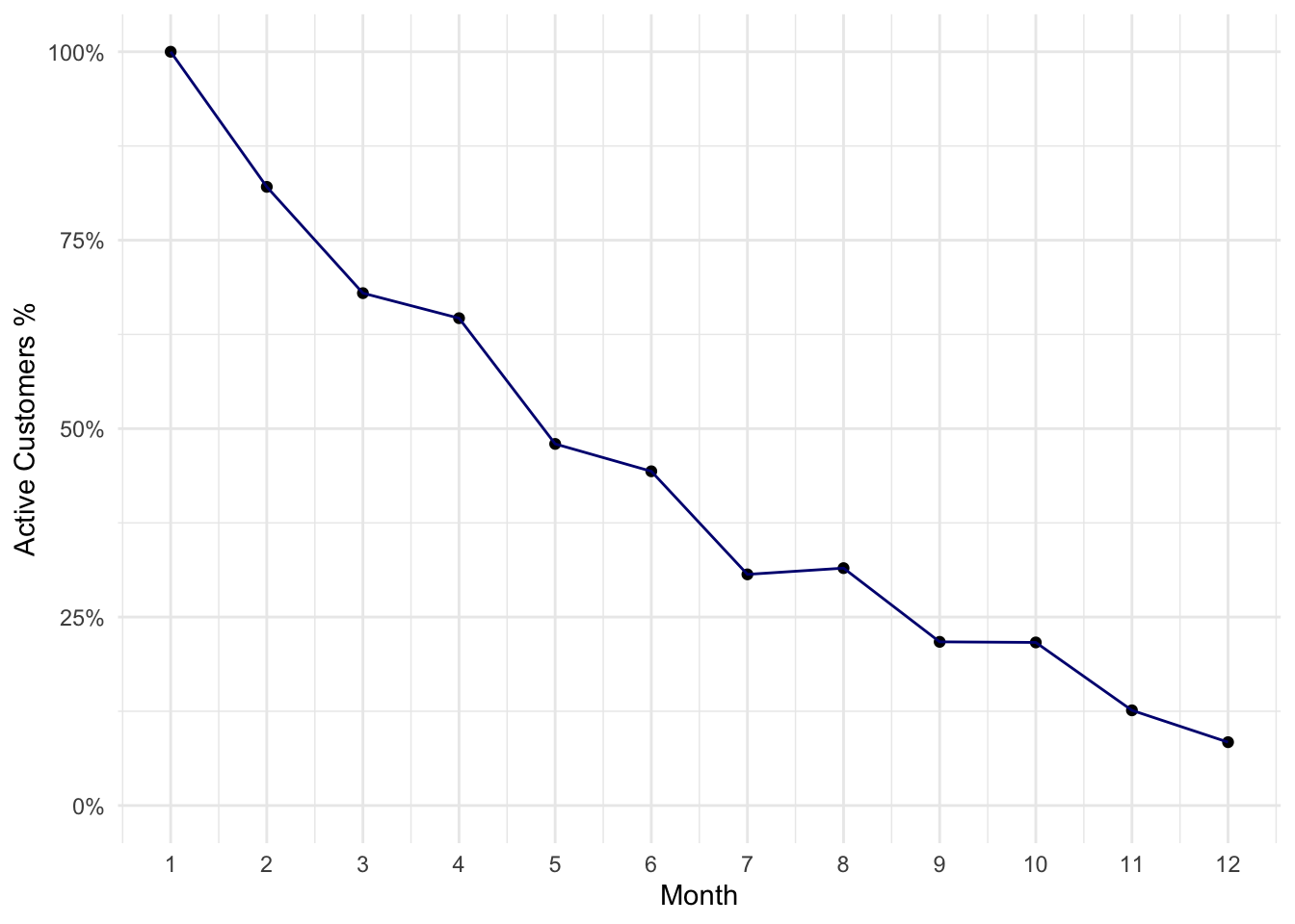

# Periodic Survival -------------------------------------------------------

# (active at period t + 1) / (active at period t)
rolling_active <- function(t) {
  
  # subset those who active at period t
  s = dat[dat[which(names(dat) == paste0("M", t))] == 1, ]
  
  # remain in the subsequent period
  r = s[which(names(s) == paste0("M", t + 1))] == 1
  
  # return
  sum(r) / nrow(s)
}

# (active at period t + 1) / (register at period t) 
rolling_retain <- function(t) {
  
  # subset those who join at period t
  s = subset(dat, join == t)
  
  # remain in the subsequent period
  r = s[which(names(s) == paste0("M", t + 1))] == 1
  
  # return
  sum(r) / nrow(s)
}

# put result into a data frame
res <- data_frame(
  ind = 1:(max(ts) - 1),
  grp_by_register_period = map_dbl(ind, rolling_retain),
  grp_by_active_period = map_dbl(ind, rolling_active)
) 

# make plot
res %>% 
  gather(var, val, -ind) %>% 
  ggplot(aes(ind, val, col = var)) + 
  geom_line() + 
  scale_color_discrete(labels = c("Group By Active Period", 
                                  "Group By Register Period")) +
  scale_x_continuous(breaks = ts) +
  scale_y_continuous(labels = scales::percent) +
  theme_minimal() +
  theme(legend.position = "bottom") +
  labs(x = "Month", y = "Retention Rate %", col = "")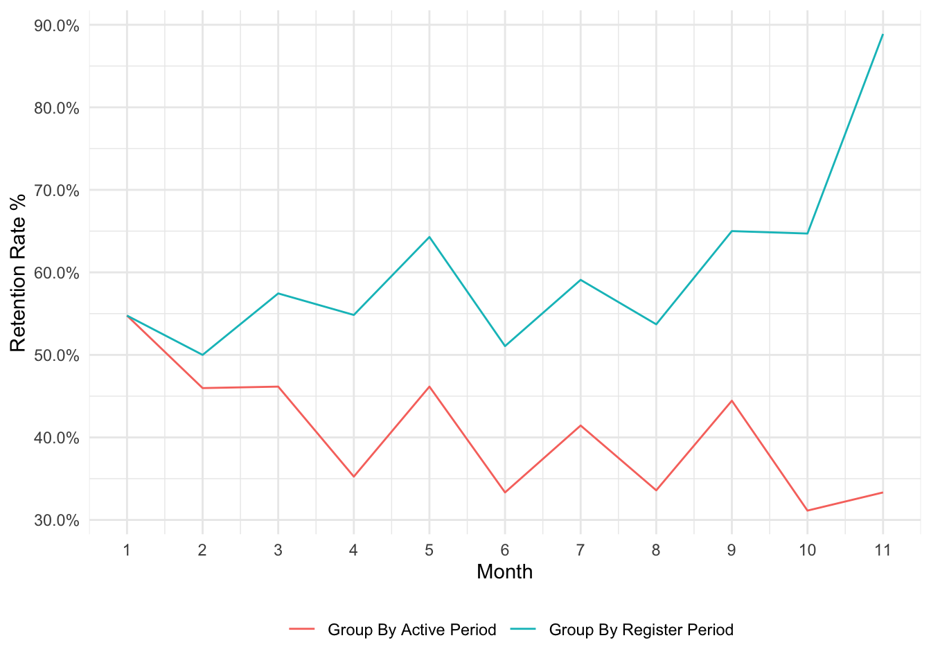

# Cohort Analysis ---------------------------------------------------------

# export to Excel to do pivot table
file <- dat %>% 
  select(-jobs) %>% 
  gather(month, active, -c(id, join)) %>% 
  mutate(month = factor(str_remove(month, "^M")))
# write_csv(file, "some/path")