Simulate Tossing Coin Game

Tossing Coin Game

Tom and Jerry play a simple game of tossing a coin. If given heads, Tom pays Jerry a dollar. Otherwise, Jerry pays Tom a dollar.

set.seed(1212)

# how many tosses?
number_of_tosses = 50

# simulate n tosses
# 1 = head, -1 = tail
(tosses <- sample(c(1, -1), size = number_of_tosses, replace = TRUE, prob = c(.5, .5)))

##  [1] -1 -1  1 -1  1 -1 -1 -1  1 -1  1  1 -1  1  1 -1 -1 -1  1 -1  1 -1 -1 -1  1
## [26] -1  1  1  1  1 -1 -1 -1  1 -1  1  1  1  1 -1 -1  1  1 -1 -1  1 -1  1  1 -1

Let’s observe some games’ progression, from the perspective of Tom.

library(purrr)

# convert game to a function
new_game <- function(n = 1) {
  tosses = sample(c(1, -1),
                   size = n,
                   replace = TRUE,
                   prob = c(.5, .5))
}

# progress of 4 different games
par(mfrow = c(2, 2))
walk(1:4, ~ {
  plot(cumsum(new_game(number_of_tosses)), type = "l", ylab = "Winnings")  
  abline(h = 0, col = "red", lty = 3)
})

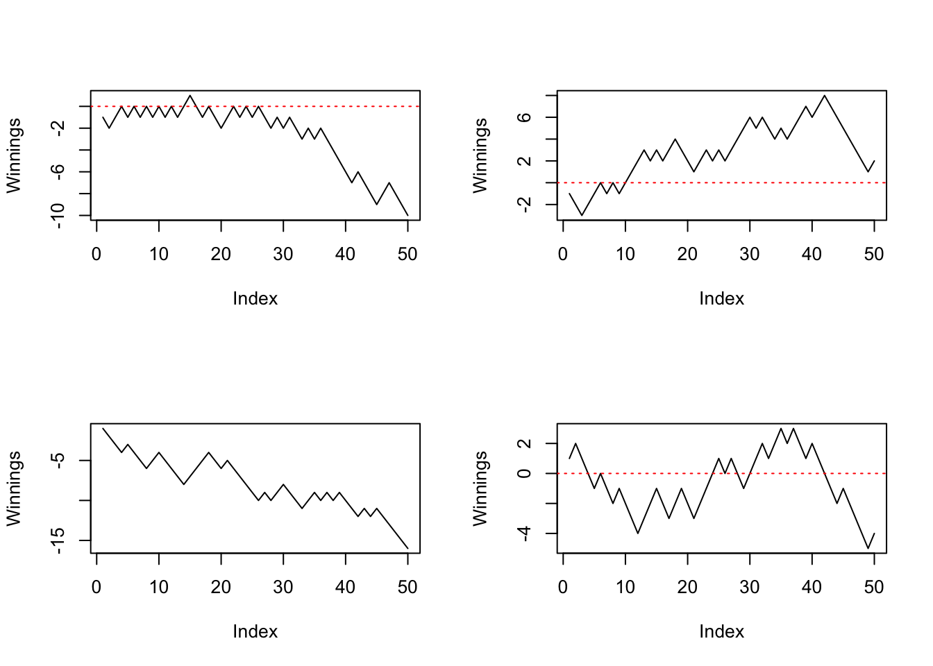
Let’s calculate the winnings distribution.

library(dplyr)
library(ggplot2)
library(ggthemes)

old <- theme_set(theme_tufte() + theme(text = element_text(family = "Menlo")))

# modify function above
new_game <- function(n = 1) {
  tosses = sample(c(1, -1),
                  size = n,
                  replace = TRUE,
                  prob = c(.5, .5))
  # return winnings
  sum(tosses)
}
# repeat many times
reps <- 10e3 %>% rerun(new_game(number_of_tosses)) %>% unlist()

# bind into data frame
reps %>%
  as_data_frame() %>%
  ggplot(aes(value)) +
  geom_histogram(binwidth = 1) +
  scale_x_discrete(limits = seq(-24, 24, 4))

## Warning: `as_data_frame()` is deprecated as of tibble 2.0.0.
## Please use `as_tibble()` instead.
## The signature and semantics have changed, see `?as_tibble`.
## This warning is displayed once every 8 hours.
## Call `lifecycle::last_warnings()` to see where this warning was generated.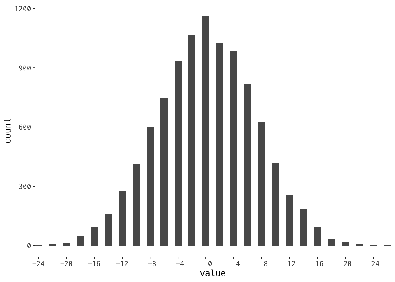

Question: Why there isn’t any odd number?

We can also calculate the chances where Tom break even, either from simulation result above, or using binomial distribution. They are pretty close.

# how many breakeven
length(which(reps == 0)) / length(reps)

## [1] 0.1163

# approx. form using binomial distribution
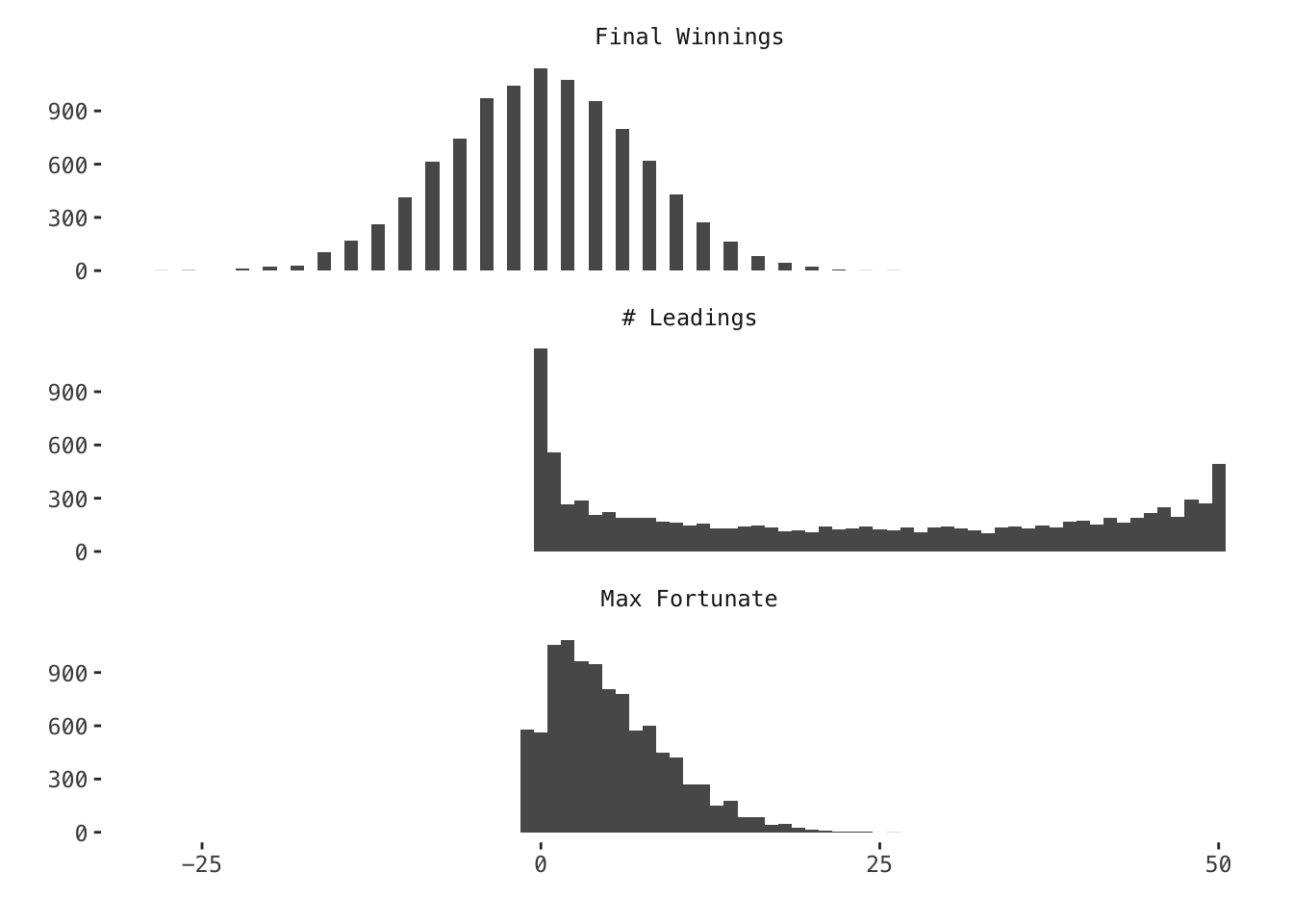
dbinom(25, size = 50, prob = 0.5) 

## [1] 0.1122752

What is the likely number of tosses Peter will be winning in a game of 50 tosses? What is the likely maximum fortune Peter will be winning in a game of 50 tosses?

library(tidyr)

# modify function above
new_game <- function(n = 1) {
  tosses = sample(c(1, -1),
                  size = n,
                  replace = TRUE,
                  prob = c(.5, .5))
  # track progress
  cum.win = cumsum(tosses)
  # return
  list(
    final = sum(tosses),
    leads = sum(cum.win > 0),
    max = max(cum.win)
  )
}
new_game(number_of_tosses)

## $final
## [1] 12
## 
## $leads
## [1] 50
## 
## $max
## [1] 13

# repeat
set.seed(1234)
reps <- 10e3 %>% rerun(new_game(number_of_tosses))

reps %>%
  bind_rows() %>%
  # collapse columns into one
  gather(var, val) %>%
  ggplot(aes(val)) +
  geom_histogram(binwidth = 1) +
  facet_wrap( ~ var, ncol = 1,
              labeller = labeller(
                var = c(final = "Final Winnings",
                        leads = "# Leadings",
                        max = "Max Fortunate")
              )) +
  labs(x = "", y  = "")